Stanford Pratical Machine Learning-神经网络

这一章主要介绍多层感知机

MLP

Handcrafted Features -> Learned Features

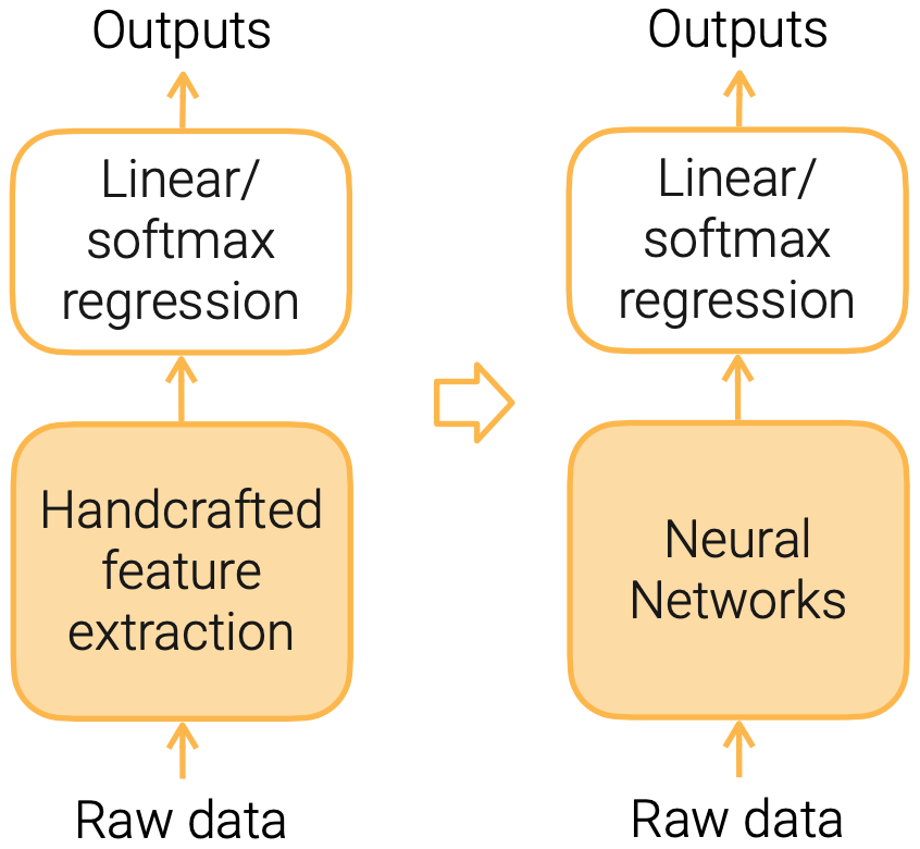
• NN usually requires more data and more computation
• NN architectures to model data structures
  • Multilayer perceptions
  • Convolutional neural networks
  • Recurrent neural networks
  • Attention mechanism
• Design NN to incorporate prior knowledge about the data

Linear Methods -> Multilayer Perceptron (MLP)

• A dense (fully connected, or linear) layer has parameters，$w\ and\ b$， it computes output $y = wx + b$

• Linear regression: dense layer with 1 output

• Softmax regression:

  • dense layer with m outputs + softmax

Multilayer Perceptron (MLP)

• Activation is a elemental-wise non-linear function
  • sigmoid and ReLU
  • It leads to non-linear models
• Stack multiple hidden layers (dense + activation) to get deeper models
• Hyper-parameters: # hidden layers, # outputs of each hidden layer
• Universal approximation theorem

Inputs -> Dense -> Activation -> Dense -> Activation -> Dense -> Outputs

Code

• MLP with 1 hidden layer
• Hyperparameter: num_hiddens

def relu(X):
  return torch.max(X, 0)

W1 = nn.Parameter(torch.randn(num_inputs, num_hiddens) * 0.01)
b1 = nn.Parameter(torch.zeros(num_hiddens))
W2 = nn.Parameter(torch.randn(num_hiddens, num_outputs) * 0.01)
b2 = nn.Parameter(torch.zeros(num_outputs))

H = relu(X @ W1 + b1)
Y = H @ W2 + b2

• Full code: http://d2l.ai/chapter_multilayerperceptrons/mlp-scratch.html

CNN

Dense layer -> Convolution layer

• Learn ImageNet (300x300 images with 1K classes) by a MLP with a single hidden layer with 10K outputs

  • It leads to 1 billion learnable parameters, that’s too big!
  • Fully connected: an output is a weighted sum over all inputs

• Recognize objects in images

  • Translation invariance: similar output no matter where the object is
  • Locality: pixels are more related to near neighbors

• Build the prior knowledge into the model structure

  • Achieve same model capacity with less # params

Convolution layer

• Locality: an output is computed from $k \times k$ input windows
• Translation invariant: outputs use the same $k \times k$ weights (kernel)
• # model params of a conv layer does not depend on input/output sizes -> n × m → k × k
• A kernel may learn to identify a pattern

Code

• Convolution with matrix input and matrix output (single channel)
• code fragment:

# both input `X` and weight `K` are matrices
h, w = K.shape
Y = torch.zeros((X.shape[0] - h + 1, X.shape[1] - w + 1))
# stride = 1
for i in range(Y.shape[0]):
	for j in range(Y.shape[1]):
		Y[i, j] = (X[I : i+h, j : j+w] * K).sum()

• Full code: http://d2l.ai/chapter_convolutionalneural-networks/conv-layer.html

• Exercise: implement multi-channel input / output convolution

Pooling Layer

池化层（汇聚层），减少对于像素级别便宜的敏感

• Convolution is sensitive to location
  • A translation/rotation of a pattern in the input results similar changes of a pattern in the output
• A pooling layer computes mean/max in windows of size k × k
• code fragment:

# h, w: pooling window height and width
# mode: max or avg
Y = torch.zeros((X.shape[0] - h + 1, X.shape[1] - w + 1))
for i in range(Y.shape[0]):
	for j in range(Y.shape[1]):
		if mode == 'max':
			Y[i, j] = X[i : i+h, j : j+w].max()
		elif mode == 'avg':
			Y[i, j] = X[i : i+h, j : j+w].mean()

• Full code: http://d2l.ai/chapter_convolutional-neural-networks/pooling.html

Convolutional Neural Networks (CNN)

• Stacking convolution layers to extract features
  • Activation is applied after each convolution layer
  • Using pooling to reduce location sensitivity
• Modern CNNs are deep neural network with various hyper-parameters and layer connections (AlexNet, VGG, Inceptions, ResNet, MobileNet)

Inputs -> Conv -> Pooling -> Conv -> Pooling -> Dense -> Outputs

RNN

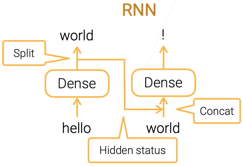
Dense layer -> Recurrent networks

• Language model: predict the next word
• Use MLP naively doesn’t handle sequence info well:

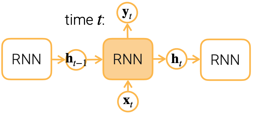
RNN and Gated RNN

• Simple RNN

• Gated RNN (LSTM, GRU): finer control of information flow
  • Forget input: suppress $x_t$ when computing $h_t$
  • Forget past: suppress $h_{t-1}$ when computing $x_t$

Code

• Implement Simple RNN, code fragment:

W_xh = nn.Parameter(torch.randn(num_inputs, num_hiddens) * 0.01)
W_hh = nn.Parameter(torch.rand(num_hiddens, num_hiddens) * 0.01)
b_h = nn.Parameter(torch.zeros(num_hiddens))

H = torch.zeros(num_hiddens)
outputs = []

for X in inputs: # `inputs` shape : (num_steps, batch_size, num_inputs)
	H = torch.tanh(X @ W_xh + H @ W_hh + b_h)
	outputs.append(H) 

• Full code at http://d2l.ai/chapter_recurrent-neural-networks/rnn-scratch.html

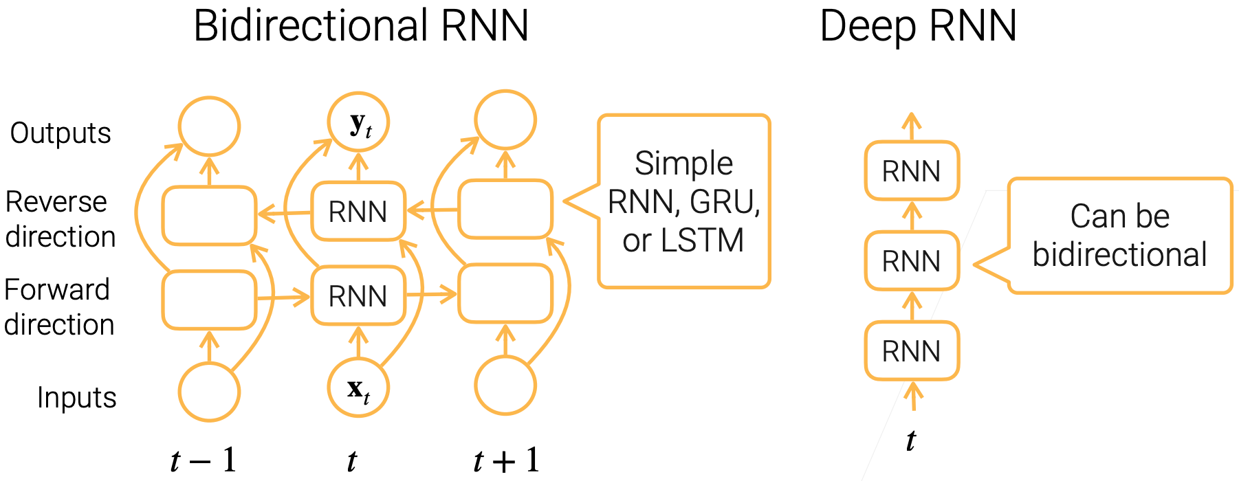
Bi-RNN and Deep RNN

Model Selections

• Tabular
  • Trees
  • Linear/MLP
• Text / speech
  • RNNs
  • Transformers
• Images / audio / video
  • CNNs
  • Transformers

Summary

• MLP: stack dense layers with non-linear activations
• CNN: stack convolution activation and pooling layers to efficient extract spatial information
• RNN: stack recurrent layers to pass temporal information through hidden state

References

1. slides